Page Title

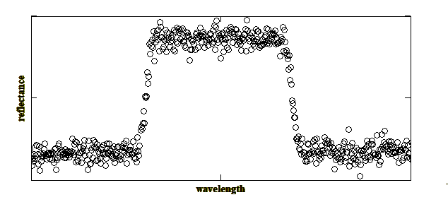
Any measurement, no matter how carefully performed will have a certain level of uncertainty attached to it. For example, if an apparently stable voltage of 1.6v is measured several times we might always obtain the same value. Now, if we add an extra digit we might find that we always measure 1.63v.

That's fine, but if we carry on with this process we will eventually reach a point when the measured voltage is different almost every time. For example, let's now measure to 5 decimal places. We might find that we now obtain the follow set of values:

1.63459, 1.63462,1.63460, 1.63457, 1.63461

The mean of these values is 1.634598 and the small-sample standard deviation is 0.000019. We would probably express the result as 1.63460 +/-0.00002.

So far so good, it's all common sense really. Moving on to a measurement parameter which is derived from a series of measurements, an example might be the spectral passband of, say, a fibre Bragg grating. Here the intensity of light reflected by the grating is measured as a function of optical wavelength. The main parameters of importance are the width of the passband, the transmission peak and the level of ripple in the passband.

In the same way that the voltage measurements varied in the above example, each data point in the grating measurement will also be subject to variation, or 'noise' as it is generally called. An example of a rather noisy measurement is shown below:

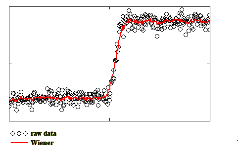
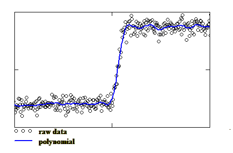
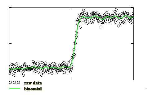
It can be seen that each of the smoothed curves follows the original data-set quite well and the steepness of the rising edge is not unduly rounded off. Any increase in the amount of smoothing by, for example, a wider fitting window for the polynomial fit or the binomial filter, or a narrower passband in the Wiener filter would result in a smoother curve but one which would fail to follow the trend of the raw data and would effectively degrade the roll-off at the edges of the passband.

Passband Calculation - Now, to calculate the width of the passband at the 50% level, known as the Full-Width at Half Maximum (FWHM), we need to determine the upper and lower levels in the profile. One very effective way of doing this is to plot a histogram of all the intensity levels and locate the positions of the centres of the peaks corresponding to the upper and lower levels. The 50% threshold is then simply the average of these two values.

The next step depends on which type of smoothing has been used. For the binomial filter and the Fourier filter the data points just above and below the threshold are found and then a simple linear interpolation (straight line fit) may be used to determine the wavelength corresponding to the 50% threshold level. For the cubic spline and the polynomial fit the edge positions at the 50% threshold can be computed directly from the coefficients of the fitted curves.

It will be appreciated that the steepness of the edges of the passband for a grating filter is an important parameter in avoiding crosstalk between adjacent channels. To specify this quantity the passband width at, say, the -20dB level is often determined as well as the -3dB (50%) level considered in this example.

Discussion - While data smoothing is an effective means of reducing the level of noise in measurement data it should be remembered that there is no real substitute for acquiring better data in the first place. Curve fitting, however, usually makes noisy data look more pleasant to the eye and indeed enables features to be seen that would otherwise be indistinguishable from the noise. The choice of smoothing algorithm, and the various filter parameters, depends very much on the particular application and what is expected from the smoothed data. For example, if the actual curve shape of the curve being measured is already known, perhaps from theoretical considerations, then it is likely that the most effective smoothing will be obtained by fitting a curve of that particular shape. An example of this is the three-term Sellmeier equation which is the standard fitting function for measured group delay data in a conventional single-mode fibre. As a general purpose filter, the binomial is perhaps the easiest to implement and it usually gives good results, but if the data points are not equally spacing then it can run into trouble and the polynomial or cubic spline filters are probably more suitable.

Binomial Smoothing - In the binomial filter each point in the dataset is replaced by a value equal to the weighted average of some of the points nearby. Each point in the binomial filter is given a weighting according to the binomial distribution so that points further from the point of interest have a decreasing effect. For example, a three point binomial filter has the following weighting coefficients: 0.25, 0.50, 0.25. The only parameter that can be chosen in binomial smoothing is the width of the smoothing window. The binomial filter can have advantages over the polynomial smoothing method in that it prevents erroneous phase shifts occurring when the polynomial fit parameters are badly chosen, but it does, however, lack the flexibility of the polynomial fit. A variation of the binomial filter is where the distribution of weights corresponds to that of a Gaussian distribution which, for a large number of points, is very similar in shape to the binomial distribution.

An example of the Binomial filter is shown as the green line in the figure below:

Polynomial Smoothing - A local nth degree polynomial fit is applied to the neighbouring datapoints surrounding a particular point in the dataset and the 'correct' value of the datapoint is taken as the value of the polynomial at that point. The polynomial fit then moves on to the next point and so a smoothed version of the data is mapped out. There are two fitting parameters for the polynomial, these are its degree, which determines how 'flexible' the fitted curve can be, and the fit window, which is the range of points on either side of the point of interest which are included in the fit. Some care has to be taken in balancing these two parameters so that the true shape of the data is followed by the curve fit but unwanted noise is smoothed out.

A particularly efficient algorithm for computing the polynomial filter has been described by Savitzky and Golay and enables rapid calculation of the polynomial coefficients and also, incidentally, their derivatives which are often useful for edge location purposes.

Another implementation of polynomial smoothing is known as the 'cubic spline' fit. This is where a series of cubic polynomials are fitted to the data such that certain conditions are met where the individual curves meet each other. These conditions are that the first and second derivatives of adjacent curves have to be equal so as to avoid discontinuities at the joints. The main fitting parameter is the width of the fit window, although there are certain conditions that also may be selected for the points at either end of the dataset to ensure stability of the curve fits in those regions.

An example of the Polynomial filter is shown as the blue line in the figure below:

Low-pass Fourier Filtering - The Fourier Transform of the dataset is first computed to give the frequency spectrum of the dataset. Higher frequencies in the spectrum generally correspond to noise in the data and these may be filtered out by multiplying the frequency spectrum by a low-pass filter so that frequencies above a certain limit are set to zero. The inverse Fourier Transform is then used to re-compute the original dataset but without the presence of noise. It should be said, however, that this method will also tend to smooth out rapid transitions in the data that are not due to noise, such as the rising and falling edges in the profile shown above. A balance has to therefore be achieved between eliminating the noise and distorting the dataset.

A frequency filter often employed as being near to optimal is known as the Wiener Filter. In this case the filter function is derived from having an approximate knowledge of both the noise frequency spectrum in the dataset and also the shape of the signal spectrum. In the example considered here the noise spectrum is fairly flat and may be approximated by a constant. The signal spectrum is also known to some extent, as the expected shape of the profile is known.

An example of applying the Wiener filter is shown as the red line in the figure below:

In order to measure the width of the passband at, say, the 50% level it is necessary to somehow minimise the effect of the noise on the measurement. The best way to do this is, of course, to reduce the noise level by more careful design of the measurement apparatus, but that's another story!

If it is observed that the noise appears to be stable and fixed with respect to its position in the profile then it is likely that the noise is not of a random nature but is, rather, coherent. This could be due to a variation in detector sensitivity across the spectrum, or maybe variations in the spectral output of the source, or due to dirt on the optics. Of course, coherent structure may be an actual feature of the sample being measured. Each of these possibilities can be investigated by making appropriate systematic checks on the apparatus.

If it is found that the noise appears to vary randomly between successive measurements, and it is not possible to reduce the noise any other way, then a good method is to take several spectral scans and compute the average. In this way the signal to noise ratio will improve as the square root of the number of measurements taken, leading to a much smoother profile.

If, after all this, the noise is still unacceptably large and makes accurate location of the edges of the passband very difficult, then artificial smoothing of the data using mathematical techniques may be employed.

There are several ways of smoothing data, a few of which are described below: